
Abstract
The present work shows that it is possible to analytically solve a general model to explain the transmission dynamics of SARS-CoV-2. First, the within-host model is described, and later a between-host model, where the coupling between them is the viral load of SARS-CoV-2. The within-host model describes the equations involved in the life cycle of SARS-CoV-2, and also the immune response; while that the between-Host model analyzes the dynamics of virus spread from the original source of contagion associated with bats, subsequently transmitted to a host, and then reaching the reservoir (Huanan Seafood Wholesale Market in Wuhan ), until finally infecting the human population.
Author Contributions
Academic Editor: Anubha Bajaj, India
Checked for plagiarism: Yes
Review by: Single-blind
Copyright © 2023 Raul isea.
 This is an open-access article distributed under the terms of the Creative Commons Attribution License, which permits unrestricted use, distribution, and reproduction in any medium, provided the original author and source are credited.
Competing interests
The authors have declared that no competing interests exist.
Citation:
Introduction
The World Health Organization (WHO) reported 27 cases with a new severe respiratory syndrome of unknown etiology from Wuhan (Hubei province) in China 1. Later identifies that it is a β-Coronavirus after sequencing the first days of January 2020 2. They originally called it 2019-nCOV, and after a month, it was renamed Severe Acute Respiratory Syndrome Coronavirus 2 (SARS-CoV-2), where the disease it produces is Covid-19. The WHO declared it an international public health emergency on January 30, 2020, and it was later declared a pandemic on March 11, 2020 3.
So far the world has faced three coronavirus associated outbreaks. .The first was called SARS-CoV-1 4, and it originated in the province of Guangdong Province in China: eight thousand cases were confirmed with a little less than eight hundred deaths in 2002 (affecting 29 countries until January 2004).The second incident was traced in Saudi Arabia, and for this reason, it was named MERS-CoV (Middle East Respiratory Syndrome Coronavirus), its first case was reported in June 2012 until November 2018, registered 2,494 cases after affecting 27 countries 5. SARS-CoV-2 has infected more than 757 million people and 6 million deaths approximately until February 23, 2023, according to Johns Hopkins University (data available at coronavirus.jhu.edu).
It is currently a public health problem. Multiple vaccines have been developed to control the spread of the disease and to reduce the number of infections recorded daily in various parts of the world. However, it is necessary to do more studies, for example, on how to reduce the application of multiple doses regimens for a person, and so on. It can probably do identification of genomic patterns capable of generating an immune response in people derived from epitopes, as has been tested in other diseases 6, 7, 8, and later can be automated with the help of specialized workflows for automatic data handling 9.
Until this is achieved, it is necessary to develop mathematical models to design the public policies necessary to contain said infections based mainly on the implementation of social distancing measures, the use of face masks, quarantine programs and vaccination campaigns, etc.
In the scientific literature, there is a wide range of mathematical models that explain, for example, the contagion dynamics in various countries without a consensus on the prediction methodology (some examples in 10, 11). Other works explain the transmission of viral particles in the environment 12, and also studies have also been carried out where they analyze the response of the immune system 13, 14. However, it is necessary to integrate all these approaches on the same time scale. This process is known as immuno-epidemiological models of infectious disease systems 15 where they are described from a cellular level to the spread in the population. This type of model has been used in the dynamics of contagion in HIV-1 with a system of six differential equations 16, 17, as well as the paper of Murillo et al 18 by studying a multiscale model to explain the Influenza infection in 2013.
The present work presents a general model to explain the transmission dynamics of SARS-CoV-2, dividing the model in two sections. We first studied the within-host scale which we will divide into two different levels. The first consists of twelve compartments to describe the life cycle of SARS-CoV-2, and later the immune response. Finally, the between-host model consists of twelve compartments to describe the transmission of the virus from the source that gave rise to the virus (bats), the host (pangolins probably), the reservoir (Huanan Seafood Wholesale Market in Wuhan), until reaching the population human where we have added a compartment to explain the environmental viral load, a key element to integrate both scales.
Mathematical model
The mathematical model describes the contagion dynamics at two different sections scales, i.e., within-host model and between-host models. Each of them is described below.
Within-host model
The within-host model include the transmission dynamics from the life cycle of SARS-CoV-2, and subsequently the model that reproduces the immune response will be explained.
SARS-CoV-2 life cycle
The virus is a single-stranded RNA virus belonging to the Coronaviridae family, Coronavirinae subfamily 19. The first reading frame, known as ORF1ab (the largest gene), occupies two-thirds of the virus sequence, approximately 28-32 kb. It is a 5’-capped and 3’-polyadenylated positive-sense single-strand RNA (+ssRNA), non-segmented and similar to the structure found in messenger RNA of eukaryotic cells.The replication of the virus begins when the S protein of SARSCoV-2 binds directly to the Angiotensin-Converting Enzyme 2 (ACE2) receptor. Once the virus has entered the host cell, it is released into the cytoplasm, starting the replication process that will give rise to non-structural proteins and also accessory proteins, with four structural proteins. The formation of RNA(-) and also replication and transcription of RNA subgenomics. These subgenomic RNAs(-) are transcribed into mRNAs(+) which encode the structural proteins S, M, E, N, and accessory proteins. During the replication process, the N protein of the virus binds to the genome, while the M protein associates with the membranes of the endoplasmic reticulum (ER). Finally, the virions are secreted by exocytosis 19.
Recently Isea and Mayo-Garc´ıa 20 have proposed the first analytical solution for the life cycle of SARS-CoV-2 according to the previous description. This model can be seen in figure 1, where it has been divided into four levels in different colors, where the first explains the cell entry, the second the genome transcription and replication, then the translation of structural and accessory proteins, and finally the assembly and eventual releases of new virions from the cell. The twelve variables that are going to describe the SARS-CoV-2 life cycle model are shown in Table 1, so the equations are simply (details in 20):

Here [Vrelease] is the concentration of viral particles that are released in the cell, and they are precisely the ones that will trigger the immune response in people, as will be explained in the next section.
Figure 1.Diagram of the life cycle of SARS-CoV-2The level that describes the cell entry is shown in blue color and indicated with number 1. The transcription and replication of the genome is in red color (number 2), while that the translation of structural and accessory proteins, and the assembly and release of virions are show in green and orange color, respectively. Only a few constants are shown in the life cycle dynamics and all the details are described in the text.
| Variable | Description | Variable | Description |
|---|---|---|---|
| [Vfree] | Free virions outside of cell | [gRNA−] | Negative sense genomic and subgenomic |
| [Vbound ] | Number of virions bound to ACE2 | [gRNA] | Positive sense ge- nomic and subgenomics RNAs |
| [Vendosome] | Number of virionsin endosomes | [N] | Concentration of Nproteins per virion |
| [gRNA+] | Numberofss-Positive sensegenomic RNA | [SP] | S+M+E per virion |
| [NSP] | Abundance of nonstructural protein populations | [N − gRNA] | Ribonucleocapsid molecules |
| [Vassemble] | Assembled virions | [Vreleased ] | Released virions |
Modelling the immune response
The immune response that is triggered in people as a result of infection by SARSCoV-2 virions has been described in various models in the scientific literature 21, 22, but most posts solve it numerically. Furthermore, recent studies have associated a storm of cytokines generated by SARS-CoV-2 such that it leads lymphocytes to the lungs in search of infection, and thus maintains the replication and transmission of the virus 23.
Of all the models available in the scientific literature, we only consider the simplest of them, as shown in
Figure 2.Diagram illustrating the immune response (see text for more details)
Figure 2, where the target cells (cells without contagion and represented by the letter T) are going to be infected (I) as a result of SARS-CoV-2 viral particles (V), so that an immune response product of antibodies is generated (A) (details in 22). The equations that describe the above process are:

Where T, I, V, and A represent target cells, infected cells, viral particles, and antibodies, respectively. The definitions of parameters will be derived directly from the work of Danchin et al 24. So both the life cycle of the virus and the dynamics of the immune response present the viral load, which is the link between them.
Between-hosts model
Figure 3 represents a model of the transmission dynamics from the possible origin of the virus associated with bats (denoted with the subscript B), then infecting an unknown host (usually associated with pangolins, abbreviated with the letter H). Later it reaches the reservoir (i.e., Wuhan market, W), until finally infecting the human population (P)
Figure 3.The Flowchart of the model proposed in this paper. The infection source is shown in blue color and it is a bats population, represented with B subscript. The host region is green and depicted with the H subscript (some bioinformatics studies indicated that could be pangolin population). The Reservoir (violet re- gion) was the Seafood Market in Wuhan. Finally, the human people are the last section and identified with the P subscript in cyan color.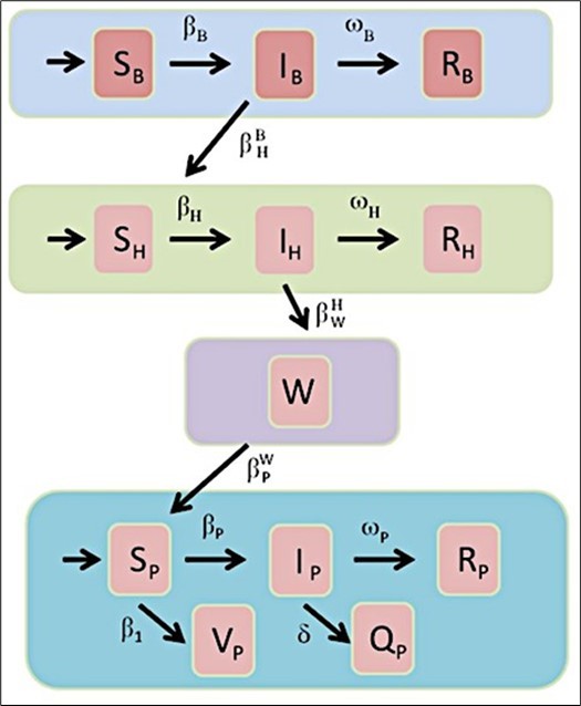
Therefore, this model that allow us to explain the transmission of the virus is given by the following differential equations:

We can observe this model is divided into twelve categories where the subscripts B, H, and P have been used to represent the bat, pangolin, and human, respectively. The Populations susceptible to contracting the virus are SB, SH, and SP, and the population infected are IB, IH, and IP. RB, RH ,and RPrepresent the recovered bat, pangolin, and human populations, and QPis the population that is in quarantine. The reservoir is denoted as W , and the last compartment is VP, which represents the environmental viral load, respectively.
The constants ΛB, ΛH and ΛP are the newborn bats, pangolins, and human, respectively. The contagion rate in bats, pangolins, and humans is given by the constants βB, βH, and βP, respectively. Also, mB, mH, and mP represent the death rate, and NB, NH and NPare the total populations of bats, pangolins, and human, respectively; ωB, ωH, and ωP are the infectious period of bats, pangolins, and human, respectively. The infection rate between bats and pangolins is given by the variable βBH, where the superscript and subscript identify the beginning and end of the rate of infection, respectively; while the contagion rate from pangolins to the reservoir is given by βHw, and βWPfrom reservoir to human. These values should be obtained by fitting the model with the collected data. Finally, εis the lifetime of the virus in the Reservoir. Given that each country maintains different policies to combat the virus, it is necessary to fit it according to infected data.
Mathematical analysis and numerical calculations
The resolution of the systems of equations have been validated in multiple scientific works 25, 26, 27, 28, so only the critical points and the eigenvalues of the system that allow us to elucidate the scenario to explain the dynamical of contagious of Covid-19.
Analysis of the within-host model
SARS-CoV-2 life cycle
The mathematical details have been recently published by Isea and Mayo-Garcia 20, where two critical points were derived as follows, noted with a letter each of the critical points obtained in each of the submodels descried above.
The first critical point
It is the trivial solution of the system and occurs when all variables are zero:

There is no contagion by the virus and therefore, there is no spread of the virus (i.e., disease-free equilibrium). The interesting of this critical point is that when calculating the Jacobian of the system and evaluating it at this critical point, The point, the eigenvalues basically depends on the constants referring to the entry of the virus into the human body.
Second critical point
The second critical point corresponds to an endemic model where the replication and transcription process of the virus can be seen before being released:

Table 2 shows the values of the constants in this system of equations, and the graphic results are shown in Figure 4 and Figure 5, where it can be seen both the contagion dynamics when it infects the cell (fig 4) as well as the number of particles that are assembled and released at the end of the SARS-CoV-2 life cycle (fig 5).
Table 2. Model parameters based on the Isea and Mayo-Garc´ıa’s models 20.| Parameter | Value | Parameter | Value |
|---|---|---|---|
| K diss | 0.61 | d SP | 0.04 |
| K bind | 12.00 | d N−gRNA | 0.12 |
| K f use | 0.50 | d endosome | 0.06 |
| K uncoat | 0.50 | K 1 | 2.10 |
| k complex | 0.40 | k 2 | 2.99 |
| K assemble | 1.00 | K 3 | 0.20 |
| K release | 8.00 | K 4 | 0.19 |
| d gRNA | 0.20 | K 5 | 37.32 |
| d NSP | 0.07 | K 6 | 4.39 |
| d gRNA | 0.10 | K 7 | 8.01 |
| d N | 0.02 | K 8 | 0.02 |
| K tr− | 3.00 | K tr+ | 1000.00 |
Figure 4.Evolution of virus transmission dynamics in the cell entry process (de- tails in 20).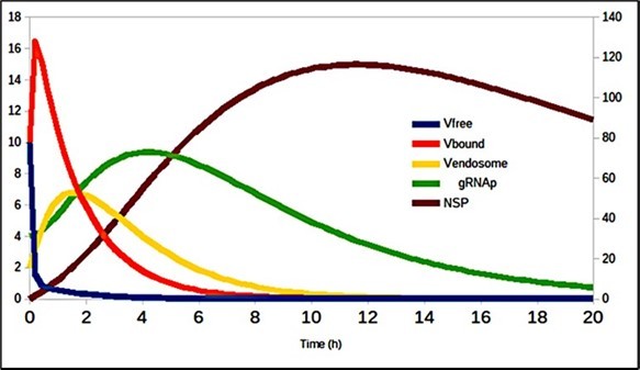
Figure 5.Number of assembled particles (Vassembled) and released (Vreleased).
Immune response
The four differential equations that allow the generation of the immune response when infected by the virus are analyzed below. This model generates three critical points (marked with a different letter for easy identification) as explained below.
The first critical point
The first critical point corresponds when there is no presence of the virus in the body (i.e., disease-free equilibrium).

Once the Jacobian evaluated at this critical point has been evaluated, two eigenvalues are obtained;

When numerically evaluating these expressions according to the value of the different parameters (Table 3), we obtain -20.28 and +2.61, that is, the system is unstable (i.e., saddle point), so further studies are necessary to identify the stability conditions of the system as well as a stability analysis in said system.
Second critical point
The second value corresponds to the case when the infection process is being generated, without generating an antibody response, described as follows:

The eigenvalues in the system are:

When evaluating these eigenvalues, the following values are obtained: -1.86E+7, and 15.53, so it is again unstable at this critical point (saddle point).
Third critical point
The last critical point is the one where the immune response is activated by the presence of antibodies, obtaining:

Unfortunately, it has not been an easy task to derive the expression of the eigenvalues for this case.
Figure 6.Immune response generated by target cells (T), cells infected (I) by SARS-CoV-2 virions (V), and antibodies generated and denoted as A.
It only remains to visualize how the immune response varies against the pres- ence of the virus as identified in Figure 6, according to the values of the parameters indicated in Table 3 (these values were obtained from the work of Danchin et al 24).
Table 3. Parameters defined in the dynamics of viral infection according to the work of Danchin et al 24| Parameter | value |
|---|---|
| µ | 9.66 |
| λT | 9.66x10⁶ |
| β | 1.28x10⁻⁶ |
| δ | 16.22 |
| c | 1.45 |
| b | 0.52 |
| σ | 0.02 |
| w | 59.74 |
| α | 9.15x10⁻⁷ |
Between-hosts model
The analytical resolution of the system of equations generates twelve different scenarios represented by the twelve critical points, where the following critical point notation (where i runs from 1 to 12) has been used to identify each of the scenarios derived in the work.
First critical point
The first critical point (CP1) is the trivial solution of the system, that is, when there are no infections in any of the populations:

This result indicates the population that may be susceptible to contracting the virus are ΛB /mB, ΛH /mHand ΛP /mPcorresponding to the populations of bats, pangolins and humans, respectively.
The next step is to determine the equilibrium conditions. The following notation has been used to describe the eigenvalues: the superscript indicates the critical point, while the subscript is the number of different eigenvalues obtained. For example, λ31corresponds to the third eigenvalue of the first critical point. By doing this, three different eigenvalues are obtained:

where three new variables (∆H, ∆B and ∆P) have been introduced indicated in Table 4 to simplify the equation in this paper. These solutions reveal that the different populations depend exclusively on each population and are not conditioned on each other.
Second critical point
The second critical point (CP2) is when only a fraction of susceptible human population without presence of the virus in the environment (W * = 0, VP*= 0) is considered:

This result reveals that it is possible to circulate the virus in the population of people who may be infected without the virus being present in the environment, infecting other people. By repeating the procedure described above, five eigenvalues are obtained:

The first two eigenvalues correspond to the equilibrium condition when the virus is not present in bats or in the host, while the last three correspond to con- ditions in the human population. These values must be adjusted with the records of contagions made in the world, as will be explained in future works.
Table 4. Definitions made to simplify mathematical expressions obtained at work.| B 0 = m B + w B + β B H |
| H 0 = m H + w H + β H W |
| P 0 = m P + w P |
| ∆B = NBmBB1 − βBΛB |
| ∆H = NHmhH1 − βHΛH |
| ∆P = NPmPP1 − βPΛP |
| E 0 = ε + β W P |
Third critical point
The third critical point (CP3) relates to the scenario when the bat population is infected, and represents the origin of the infection in the human population, so that the host can simply indicate the fraction of people susceptible to such disease, and described by the following equations:

It should be noted that the host population that can be infected by the virus depends directly on the rate of infection of the bat. The eigenvalues obtained are:

The last eigenvalues are a combination of conditions between the bat and host populations, and the equilibrium conditions depend on the values ∆B and ∆H. Actually, these values should not be easy to obtain because there are still many questions about how the virus affects the human population.
Fourth critical point
The fourth critical point (CP4) represents the scenario when the bat population and the human population are infected, without the host or the environment presenting the virus.

Where the new variables indicated in this critical point are listed in Table 4. The six eigenvalues in this scenario are:

Expressions of the combinations between species are already beginning to be obtained, which complicates the obtaining of said equations.
Fifth critical point
The fifth critical point (CP5 ) corresponds to the case when the population of pangolins is infected and the virus is also in the Reservoir, so a part of the human population is susceptible to contracting this disease, that is:

This solution reveals how the environment (W* ) plays an important role in the human population that can contract this disease. The four eigenvalues are:

As can be seen above, the first two eigenvalues depend exclusively on the parameters of the pangolins, then on the bats, and finally the last is a combination of the parameters between the host and human people.
Sixth critical point
The sixth critical point (CP6 ) corresponds to the case when bat populations and humans are infected, that is:

The eigenvalues from this critical point have not been easy to obtain.
Seventh critical point
The seventh critical point (CP7) corresponds to the case when the virus is present in bats, pangolins, and in the reservoir.

It should be noted that the human population that is susceptible to contracting the virus depends significantly on the reservoir. Only we can calculate, the eigenvalues corresponding to the bat population.

Eighth critical point
The last critical point (CP8) corresponds to the case when the three populations are infected by Covid-19, without being present at V*P = 0, and this result should be analyzed in more detail in the future .
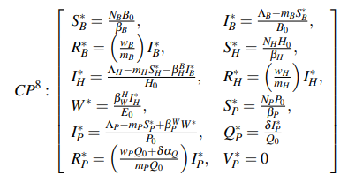
This critical point is when everyone is infected, and unfortunately it has not been possible to determine the eigenvalues for this system.
Ninth critical point
This critical point (CP9) corresponds to the case when the human population is present the virus, where VP* ≠ 0, and should be the scenario capable of describing the current transmission of the virus in different parts of the world.

This scenario tells us how the virus is transmitted in the human population once it has been infected by the environment.
Tenth critical point

Eleventh critical point

Last critical point
The last critical point is when the virus circulates and is infecting all species. It is the most general possible model that can explain the spread of the virus from its origin.

This scenario is one where the virus is transmitted between all species. Unfortunately it has not been easy to derive the eigenvalues.
It only remains to indicate, as an example, some of the values of the constants used in the last equations. These values can be seen in a study carried out by Isea 28 after adjusting the data according to the contagion data present in Australia, using a least squares adjustment, where there is infection in the population of neither bats nor pangolins. The values obtained were: β PW = 1.708, βP = 1.215, ωP = 0.001, ΛP = 81.212, µ = 1.100, ε = 0.001 (setting the mP value to 0.0000456). The value of VP must be adjusted with experimental data under a range of hypotheses that will be presented in a future work.
Conclusion
In the present work, a mathematical model has been proposed to study the transmission dynamics of Covid-19 from two different scales where the viral load of the virus is the key to unifying both these time scales. The advantage of this model is that it is possible to focus on a particular study scheme derived directly from the equilibrium conditions of the system, that is, there is a mathematical basis that justifies the existence of said scenario based on the critical points derived in the work. It should be pinpointed that all the models have been described with a deterministic model and the conditions to reach equilibrium have been obtained in most of them. In the next publication, the between-host model will be analyzed considering the sensitivity analysis and also the measures of social distancing and how quarantine affects the dynamics of contagion will be described.
Acknowledgments
The author appreciates the unconditional help of Rafael Mayo-Garcia when reading this work immersed in a sea of differential equations, and also Jesus Isea for reading and helping me with the preparation of this manuscript.
Data Availability
Data available within the article.
References
- 1.American Pan. (2020) Health Organization / World Health Organization. Epidemiological Alert: Novel coronavirus (nCoV). , Washington, D.C.: PAHO/WHO; 16.
- 2.Wu F, Zhao S, Yu B, Y M Chen, Wang W et al.A new coronavirus associated with human respiratory disease in China. , Nature 579(2020), 265-269.
- 4.R H Xu, J F He, M R Evans, G W Peng, H E Field et al.Epidemiologic clues to SARS origin in China. , Emerg. Infect.Dis 10(2004), 10301037-10.
- 5.Mostafa A, Kandeil A, Shehata M, R El Shesheny, A M Samy et al.Middle East Respiratory Syndrome Coronavirus (MERS-CoV):. , State of the Science, Microorganisms 8(2020), 991-10.
- 6.Isea R.Identificacion de once candidatos vacunales potenciales contra la ´malaria por medio de la Bioinformatica. , Vaccimonitor 19(2010), 15-19.
- 7.Isea R.Mapeo computacional de ep´ıtopos de celulas B presentes en el virus ´ del dengue. , Rev. Inst. Nac. Hig. Rafael Rangel 44(2013), 25-29.
- 8.Isea R.Quantitative computational prediction of the consensus B-cell epitopes of 2019-nCoV. , Journal of Current Viruses and Treatment Methodologies 1(2020), 42-47.
- 9.Isea R, Montes E, A J Rubio-Montero, Mayo-Garcia R. (2009) Computational challenges on Grid Computing for workflows applied to PhylogenyInternational Work-Conference on Artificial Neural Networks. 1130-1138.
- 10.Isea R.Characterizing the Dynamics of Covid-19 Based on Data. , Journal of Current Viruses and Treatment Methodologies 1(2021), 25-30.
- 11.A S Deif, S A El-Naggar.Modeling the COVID-19 spread, a case study of Egypt. , Journal of the Egyptian Mathematical Society 29(2021), 13-10.
- 12.Dragone R, Licciardi G, Grasso G, C Del Gaudio, Chanussot J.Analysis of the Chemical and Physical Environmental Aspects that Promoted the Spread of SARS-CoV-2 in the Lombard Area. International journal of environmental research and public health. 18(2021), 1226-10.
- 13.S Q Du, Yuan W.Mathematical modeling of interaction between innate and adaptive immune responses in COVID-19 and implications for viral pathogenesis. , Journal of medical virology 92(2020), 16151628-10.
- 14.Ghostine R, Gharamti M, Hassrouny S, Hoteit I.Mathematical Modeling of Immune Responses against SARS-CoV-2 Using an Ensemble Kalman Filter. , Mathematics 9(2021), 2427-10.
- 15.X Z Li, Gao S, Y K Fu, Martcheva M.Modeling and Research on an Immuno-Epidemiological Coupled System with Coinfection. , Bull. Math Biol 83(2021), 116-10.
- 16.Dorratoltaj N, Nikin-Beers R, S M Ciupe, S G Eubank, K M Abbas. () Multi-scale immunoepidemiological modeling of within-host and betweenhost HIV dynamics: systematic review of mathematical models. , PeerJ 5(2017), 3877.
- 17.Xue Y, Xiao Y.Analysis of a multiscale HIV-1 model coupling withinhost viral dynamics and between-host transmission dynamics. , Mathematical Biosciences and Engineering 17(2020), 6720-6736.
- 18.L N Murillo, M S, A S Perelson.Towards multiscale modeling of influenza infection. , Journal of theoretical biology 332(2013), 267290-10.
- 19.Kumar S, Nyodu R, V K Maurya, S K, Morphology.. Genome Organization, Replication, and Pathogenesis of Severe Acute Respiratory Syndrome Coronavirus 2 (SARS-CoV-2), Coronavirus Disease 2019 (COVID-19): Epidemiology, Pathogenesis, Diagnosis, and Therapeutics 2331-10.
- 20.Isea R, Mayo-Garc´ıa R.First analytical solution of intracellular life cycle of SARS-CoV-2. , Journal of Model Based Research 1(2022), 6-12.
- 21.Alzahrani T.Spatio-Temporal Modeling of Immune Response to SARS-CoV-2. , Infection. Mathematics 9(2021), 3274-10.
- 22.Chowdhury S M E K, J T Chowdhury, S F Ahmed, Agarwal P, Badruddin S Kamangar I A.Mathematical modelling of COVID-19 disease dynamics: Interaction between immune system and SARS-CoV-2 within host. , AIMS Mathematics 7(2022), 2618-2633.
- 23.R F, A B Pigozzo, Bonin C R B, Quintela B, L T Pompei et al.. A Validated Mathematical Model of the Cytokine Release Syndrome in Severe COVID-19, Front. Mol. Biosci. 8(2021),639423. Doi: 10.2289/fmolb 2021-639423.
- 24.Danchin A, Pagani-Azizi O, Turinici G, Yahiaoui G. (2020) COVID-19 adaptive humoral immunity models: weakly neutralizing versus antibodydisease enhancement scenarios. 2020-10.
- 25.Isea R, K E Lonngren.Toward an early warning system for Dengue, Malaria and Zika in Venezuela. , Acta Scientific Microbiology 1(2018), 30-32.
- 26.Isea R.A preliminary model to describe the transmission dynamics of Covid-19 between two neighboring cities or countries. medRxiv preprint.Doi:. 10-1101.